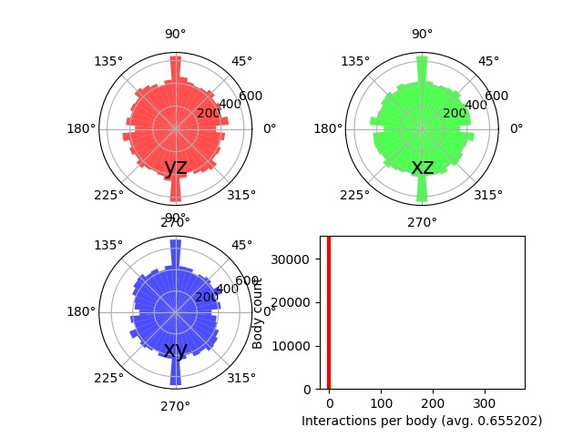
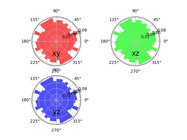
The distribution of contact normal direction and contact normal force are not uniform after isotropic consolidation

After isotropic consolidation, I check the contact normal direction and contact normal force distribution which should be evenly distributed in all directions, and I found they are not uniform. I don't know what's wrong, can you help me, thank you!
1. The code of isotropic consolidation is as follows:
 ##______________ First section, generate sample_________

from __future__ import print_function
from yade import pack, qt, plot
from math import *
import matplotlib; matplotlib.rc('axes',grid=True)
import pylab

nRead=readParamsFromTable(
        ## model parameters
        num_spheres=40000,
        targetPorosity= .33,
        confiningPressure=-50000,
        ## material parameters
        compFricDegree=25,#contact friction during the confining phase
        finalFricDegree=30,#contact friction during the deviatoric loading
        young=2e8,
        poisson=.2,
        density=2600,
        alphaKr=7.5,
        alphaKtw=0,
 competaRoll=.1,
        finaletaRoll=.1,
        etaTwist=0,
        normalCohesion=0,
        shearCohesion=0,
        ## fluid parameters
        fluidDensity=1000,
        dynamicViscosity=.001,
        ## control parameters
        damp=0,
        stabilityThreshold=.001,
        ## output specifications
        filename='suffusion',
        unknowOk=True
)

from yade.params.table import *

mn,mx=Vector3(0,0,0),Vector3(0.03,0.03,0.03)
psdSizes=[0.00042,0.0005,0.00208,0.0024]
psdCumm=[0.0,0.35,0.35,1.0]
# create materials for spheres
#shear strength is the sum of friction and adhesion, so the momentRotationLaw=True
O.materials.append(CohFrictMat(alphaKr=alphaKr,alphaKtw=alphaKtw,density=density,etaRoll=competaRoll,etaTwist=etaTwist,frictionAngle=radians(compFricDegree),momentRotationLaw=True,normalCohesion=normalCohesion,poisson=poisson,shearCohesion=shearCohesion,young=young,label='spheres'))
O.materials.append(FrictMat(young=young,poisson=poisson,frictionAngle=0,density=0,label='walls'))
walls=aabbWalls([mn,mx],thickness=0,material='walls')
wallIds=O.bodies.append(walls)
# generate particles packing
sp=pack.SpherePack()
sp.makeCloud(mn,mx,psdSizes=psdSizes,psdCumm=psdCumm,distributeMass=True,num=num_spheres,seed=1)
sp.toSimulation(material='spheres')

O.engines=[
        ForceResetter(),
        InsertionSortCollider([Bo1_Sphere_Aabb(),Bo1_Box_Aabb()]),
        InteractionLoop(
            [Ig2_Sphere_Sphere_ScGeom6D(),Ig2_Box_Sphere_ScGeom()],
            [Ip2_FrictMat_FrictMat_FrictPhys(),Ip2_CohFrictMat_CohFrictMat_CohFrictPhys(label='contact',setCohesionNow=False,setCohesionOnNewContacts=False)],
            [Law2_ScGeom_FrictPhys_CundallStrack(),Law2_ScGeom6D_CohFrictPhys_CohesionMoment(useIncrementalForm=True,always_use_moment_law=True)],
 ),
        #GlobalStiffnessTimeStepper(active=1,timeStepUpdateInterval=100,timestepSafetyCoefficient=0.8),
        TriaxialStressController(label='triax',
            # specify target values and whether they are strains or stresses
            goal1=confiningPressure,goal2=confiningPressure,goal3=confiningPressure, stressMask=7,
            # type of servo-control, external walls compaction
            internalCompaction=False,
            thickness=0,
            ),
        NewtonIntegrator(damping=0)
]

qt.View()

O.dt=0.5*PWaveTimeStep()
import sys

while True:
    O.run(1000,True)
    unb=unbalancedForce()
    print('unbalanced force:',unb,' mean stress: ',triax.meanStress)
    if unb<stabilityThreshold and abs((confiningPressure-triax.meanStress)/confiningPressure)<0.001:
        break

# reaching a specified porosity precisely
while triax.porosity>targetPorosity:
    compFricDegree=0.95*compFricDegree
    setContactFriction(radians(compFricDegree))
    print('Friction:',compFricDegree,'porosity:',triax.porosity)
    sys.stdout.flush()
    while True:
        O.run(500,True)
        unb=unbalancedForce()
        if unb<stabilityThreshold and abs((confiningPressure-triax.meanStress)/confiningPressure)<0.001:
            break

# check the position of spheres
maxX=O.bodies[1].state.pos[0]
minX=O.bodies[0].state.pos[0]
maxY=O.bodies[3].state.pos[1]
minY=O.bodies[2].state.pos[1]
maxZ=O.bodies[5].state.pos[2]
minZ=O.bodies[4].state.pos[2]
ball_out_of_wall=list()
for b in O.bodies:
    if b.state.pos[0]>maxX or b.state.pos[0]<minX:
        ball_out_of_wall.append(b.id)
        print('the walls or balls are moving too fast, the time step is too big')
    elif b.state.pos[1]>maxY or b.state.pos[1]<minY:
        ball_out_of_wall.append(b.id)
        print('the walls or balls are moving too fast, the time step is too big')
    if b.state.pos[2]>maxZ or b.state.pos[2]<minZ:
        ball_out_of_wall.append(b.id)
        print('the walls or balls are moving too fast, the time step is too big')
print(ball_out_of_wall)

# change the contact parameters to the final calibration value
setContactFriction(radians(finalFricDegree))
for b in O.bodies:
    b.mat.etaRoll=finaletaRoll
for i in O.interactions:
    i.phys.etaRoll=finaletaRoll

O.save('compactedState'+filename+'3.yade.gz')
print('Compacted state saved')
binsSizes, binsProc, binsSumCum=psd(bins=20,mass=True)
pylab.semilogx(binsSizes, binsProc,label='Mass PSD of (free) %d random spheres'%len(binsSizes))
pylab.show()

2. The code of contact normal distribution is as follows:
O.load('compactedStatesuffusion3.yade.gz')
def plotdirections(aabb=(),mask=0,bins=20,numHist=True,noShow=False,sphSph=False):
    """Plot 3 histograms for distribution of interaction directions, in yz,xz and xy planes and
    (optional but default) histogram of number of interactions per body. If sphSph only sphere-sphere interactions are considered for the 3 directions histograms.

    :returns: If *noShow* is ``False``, displays the figure and returns nothing. If *noShow*, the figure object is returned without being displayed (works the same way as :yref:`yade.plot.plot`).
    """
    import pylab,math
    from yade import utils
    for axis in [0,1,2]:
        d=utils.interactionAnglesHistogram(axis,mask=mask,bins=bins,aabb=aabb,sphSph=sphSph)
        fc=[0,0,0]
        fc[axis]=1.
        subp=pylab.subplot(220+axis+1,polar=True)
        theta1=d[0]
        theta2=[x+math.pi for x in theta1]
        theta=theta1+theta2
        radii=d[1]
        radii+=radii
        # 1.1 makes small gaps between values (but the column is a bit decentered)
        pylab.bar(theta,radii,width=math.pi/bins,fc=fc,alpha=.7,label=['yz','xz','xy'][axis])
        #pylab.title(['yz','xz','xy'][axis]+' plane')
        pylab.text(.5,.25,['yz','xz','xy'][axis],horizontalalignment='center',verticalalignment='center',transform=subp.transAxes,fontsize='xx-large')
    if numHist:
        pylab.subplot(224,polar=False)
        nums,counts=utils.bodyNumInteractionsHistogram(aabb if len(aabb)>0 else utils.aabbExtrema())
        avg=sum([nums[i]*counts[i] for i in range(len(nums))])/(1.*sum(counts))
        pylab.bar(nums,counts,fc=[1,1,0],alpha=.7,align='center')
        pylab.xlabel('Interactions per body (avg. %g)'%avg)
        pylab.axvline(x=avg,linewidth=3,color='r')
        pylab.ylabel('Body count')
    if noShow: return pylab.gcf()
    else:
        pylab.savefig('fig1.jpg')
        pylab.ion()
        pylab.show()

plotdirections(sphSph=True)

3. The code of contact normal force distribution is as follows:
import pylab,math

O.load('compactedStatesuffusion3.yade.gz')

nBins=20

def contact_normal_force_distribution(nBins=20):
    '''calculate the contact normal force distribution

    param nBins: the number of histograms
    return:
           *
    '''
    contact_normal_force_XY=[0 for i in range(nBins)]
    contact_normal_force_XZ=[0 for i in range(nBins)]
    contact_normal_force_YZ=[0 for i in range(nBins)]
    contact_nXY=[0 for i in range(nBins)]
    contact_nXZ=[0 for i in range(nBins)]
    contact_nYZ=[0 for i in range(nBins)]
    # use only sphere-sphere contacts
    for i in O.interactions:
        if not isinstance(O.bodies[i.id1].shape,Sphere):
            continue
        if not isinstance(O.bodies[i.id2].shape,Sphere):
            continue
        contact_normal=i.geom.normal
        fn=i.phys.normalForce.norm()
        angleXY=atan2(contact_normal[1],contact_normal[0])
        angleXZ=atan2(contact_normal[2],contact_normal[0])
        angleYZ=atan2(contact_normal[2],contact_normal[1])
        if angleXY<0:
            angleXY=+math.pi
        if angleXZ<0:
            angleXZ=+math.pi
        if angleYZ<0:
            angleYZ=+math.pi
        nXY=int(angleXY/math.pi*nBins)
        nXZ=int(angleXY/math.pi*nBins)
        nYZ=int(angleXY/math.pi*nBins)
        print(nXY,nXZ,nYZ)
        if nXY==nBins:
            nXY=nBins-1
        if nXZ==nBins:
            nXZ=nBins-1
        if nYZ==nBins:
            nYZ=nBins-1
        contact_normal_force_XY[nXY]+=fn
        contact_normal_force_XZ[nXZ]+=fn
        contact_normal_force_YZ[nYZ]+=fn
        contact_nXY[nXY]+=1
        contact_nXZ[nXZ]+=1
        contact_nYZ[nYZ]+=1
    for i in range(nBins):
        contact_normal_force_XY[i]=contact_normal_force_XY[i]/contact_nXY[i]
        contact_normal_force_XZ[i]=contact_normal_force_XZ[i]/contact_nXZ[i]
        contact_normal_force_YZ[i]=contact_normal_force_YZ[i]/contact_nYZ[i]
    return contact_normal_force_XY, contact_normal_force_XZ, contact_normal_force_YZ, contact_nXY, contact_nXZ, contact_nYZ

contact_normal_force_XY, contact_normal_force_XZ, contact_normal_force_YZ, contact_nXY, contact_nXZ, contact_nYZ = contact_normal_force_distribution(nBins=nBins)

theta1=[0 for i in range(nBins)]
for i in range(nBins):
    theta1[i]=i*math.pi/nBins+math.pi/(2*nBins)

theta2=[x+math.pi for x in theta1]
theta=theta1+theta2

contact_normal_force_XY+=contact_normal_force_XY
contact_normal_force_XZ+=contact_normal_force_XZ
contact_normal_force_YZ+=contact_normal_force_YZ

contact_normal_force=list()
contact_normal_force.append(contact_normal_force_XY)
contact_normal_force.append(contact_normal_force_XZ)
contact_normal_force.append(contact_normal_force_YZ)

for axis in [0,1,2]:
    fc=[0,0,0]
    fc[axis]=1.
    subp=pylab.subplot(220+axis+1,polar=True)
    pylab.bar(theta,contact_normal_force[axis],width=math.pi/nBins,fc=fc,alpha=.7,label=['xy','xz','yz'][axis])
    pylab.text(.5,.25,['xy','xz','yz'][axis],horizontalalignment='center',verticalalignment='center',transform=subp.transAxes,fontsize='xx-large')
pylab.savefig('Fig_contact_normal_force_Distribution'+str(axis)+'.jpg')
pylab.ion()
pylab.show()

The figure links of contact normal distribution and contact normal force distribution are as follows:
1. https://i.loli.net/2021/09/02/Y3nIWrmTx2FLfUc.jpg
2. https://i.loli.net/2021/09/02/oTCZmLUqjkaVB79.jpg