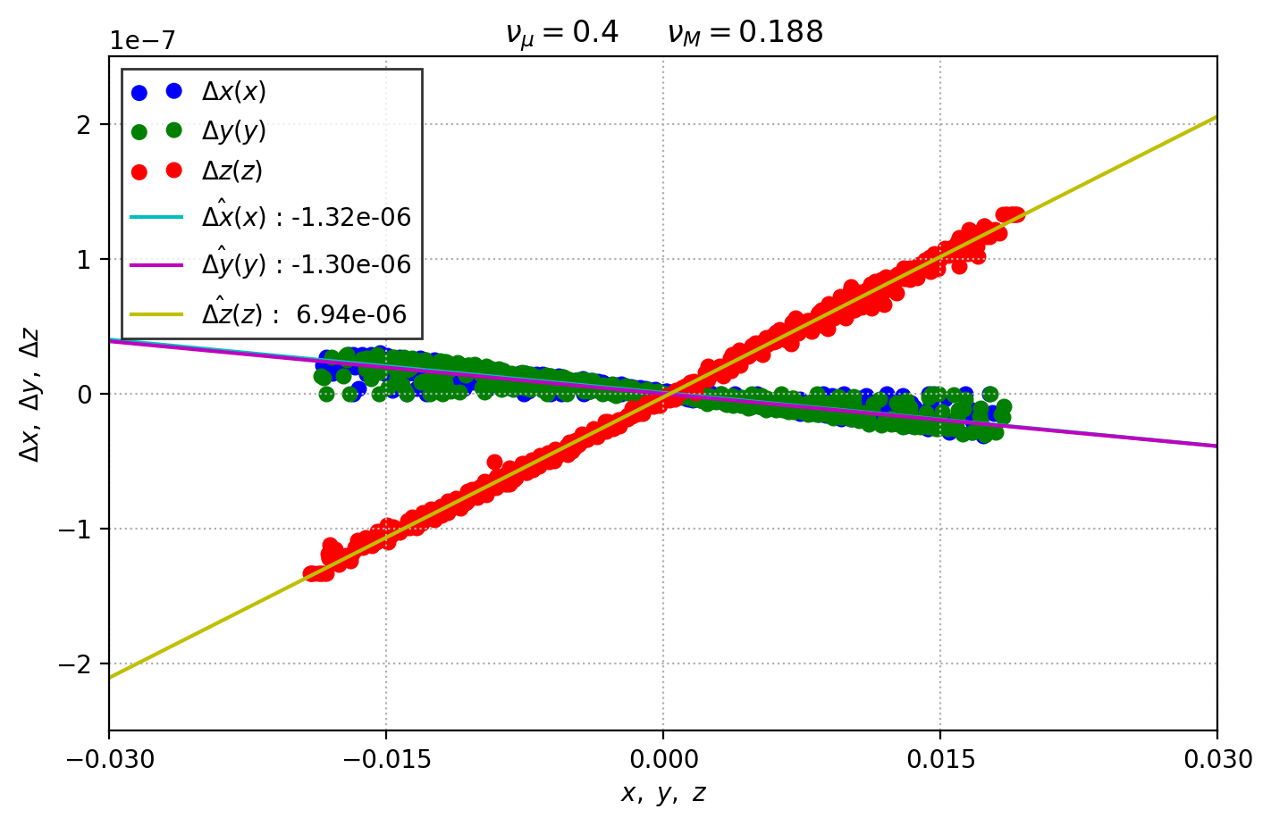
CpmMat elastic calibration difficulty

Did you visually check whether your lateralStrain = f(axialStrain) curves change when you change CpmMat.poisson ?

This should be the case, provided that CpmMat model (which I do not know) is similar enough to FrictMat / FrictPhys in this aspect.

I did, indeed. Below there are two simulations using the code above, one using poisson=0.1 and another with poisson=0.4, the curves based on Šmilauer's thesis can be found in the following links:

poisson = 0.1 ⇒ https://user-images.githubusercontent.com/19715340/74239131-fb78a200-4cb5-11ea-89c6-bfb86774663b.png
poisson = 0.4 ⇒ https://user-images.githubusercontent.com/19715340/74239098-ea2f9580-4cb5-11ea-9281-8102668205d6.png

As you can see, by changing the poisson value, the obtained macro value remained the same.

Hi,

> even though I change in the CpmMat the values of ... 'poisson'

in what range?

> I am currently trying to make the elastic calibration
> epsCrackOnset=1e-5

if you are interested in elastic calibration, set parameters influencing INELASTIC behavior such that the model remain elastic

> As you can see, by changing the poisson value, the obtained macro value remained the same.

as you can see, by changing the poisson value, the obtained macro value DID NOT remain the same.
Please provide what a why did you expect

cheers
Jan

Hello and thanks for the reply!

> in what range?

Young was varied between 20 and 100 GPa and Poisson was varied between 0.05 and 0.9 for these inicial calibration tests

>if you are interested in elastic calibration, set parameters influencing INELASTIC behavior such that the model remain elastic

I had tested some values on this parameter and as it did not influence the obtained value, I kept it 1e-5, I was wrong.

But now ran a simulation using 1e-1 and 1e0, the value of Poisson changed from 0.187 to ≃ 0.258 when moving epsCrackOnset from 1e-5 to 1e-1 but didn't change between the last two (1e-1 to 1e0), so I guess in this case it's way safer to assume this parameter is not influencing anymore, but yet the micro poisson didn't change much

Is the range of the other parameters I'm using way off to have an actual effect?

>as you can see, by changing the poisson value, the obtained macro value DID NOT remain the same.
>Please provide what a why did you expect

The element position was obtained for any timestep in which the material behavior is within the elastic domain and then compared with the initial position in order to find the deformation in that region, then, based on the formula nu = (-0.5(ex+ey))/ez, Poisson modulus was computed.

Regarding the "the value did remain the same", that graph was computed on a single timestep, if I take the average, are equal up to 4 decimal values. I agree the shown method was a poor one, hence I moved to obtaining a linear regress of the computed strains and the results are now more reliable than the former one.

In this new evaluation, the value for epsCrackOnset used was 1e-1, Micro Young 50e9 and Micro Poisson 0.2 or 0.4. The results are displayed below:

Micro Poisson = 0.2 ⇒ https://user-images.githubusercontent.com/19715340/74276747-0c94d380-4cf5-11ea-8a54-c9fcc8ce6e6e.png
Micro Poisson = 0.4 ⇒ https://user-images.githubusercontent.com/19715340/74276830-3b12ae80-4cf5-11ea-9acd-23363186a653.png

What I expected was for the values to change based on the input young and poisson but the value I'm measuring so far is kind of static when varying the elastic parameters. The reason of what I'm looking for is that Macro Young is directly related to the Micro Young whereas Macro Poisson is a function of Micro Young and Micro Poisson.

Best regards!

> Is the range of the other parameters I'm using way off to have an actual effect?

set epsCrackOnset and sigmaT to arbitrary large values (like 1e99)

please try your test with these values and let us know.

Also see [1,2] discussing similar topic.

cheers
Jan

[1] https://answers.launchpad.net/yade/+question/670047
[2] https://answers.launchpad.net/yade/+question/685862

Hello again and thanks for the reply.

>set epsCrackOnset and sigmaT to arbitrary large values (like 1e99)

I ran some simulations using 1e99 and looks like this solved the problem, now Macro Poisson is varying with the Micro value.
Low kT/kN values are now behaving like expected based on Šmilauer's thesis (e.g. kT/kN=0 ⇒ v≃0.259)

Thank you for the support, I'll continue now towards the inelastic part of the calibration.

Best regards!

Hello everyone,

I have managed to plot vary the values as described on my last post but now I face another problem: "yade" and "yade-batch" yield different results.

When I compute Poisson modulus with batch, the values obtained are akin to those found on Šmilauer's thesis, but if I run the simulations manually the values will differ.

My script can be found below:

###############################################
#!/usr/bin/python
# -*- coding: utf-8 -*-
from yade import plot,pack,timing
import time, sys, os, copy, numpy as np

savedir = './elastic_validation/'

# default parameters or from table
readParamsFromTable(
 young = 66e9,
 poisson = 0.1,

 sigmaT=1e99,
 #frictionAngle=atan(0.8),
 epsCrackOnset=1e99,
 relDuctility=1e99,
 intRadius=1.5,
 dtSafety=.1,
 damping=0.8,
 strainRateTension=.005,
 strainRateCompression=.5,
 setSpeeds=True,
 # 1=tension, 2=compression (ANDed; 3=both)
 doModes=1,

 specimenLength=.039850,
 specimenRadius=.019875,
 sphereRadius=0.75e-3,

 # isotropic confinement (should be negative)
 isoPrestress=0,
 noTableOk=True,

 n=100
)

from yade.params.table import *
if 'description' in list(O.tags.keys()): O.tags['id']=O.tags['id']+O.tags['description']

print(young, poisson)
# make geom; the dimensions are hard-coded here; could be in param table if desired
# z-oriented hyperboloid, length 20cm, diameter 10cm, skirt 8cm
# using spheres 7mm of diameter
concreteId=O.materials.append(
  CpmMat(
   young=young,
   #frictionAngle=frictionAngle,
   poisson=poisson,
   density=6420,
   sigmaT=sigmaT,
   relDuctility=relDuctility,
   epsCrackOnset=epsCrackOnset,
   #isoPrestress=isoPrestress,
   neverDamage=True,
   )
  )

#sps=SpherePack()

#sp=pack.randomDensePack(pack.inAlignedBox((0,0,0),(specimenLength,specimenLength,specimenLength)),
sp=pack.randomDensePack(pack.inCylinder((0,0,-.5*specimenLength),(0,0,.5*specimenLength),specimenRadius),
      spheresInCell=5000,
      radius=sphereRadius,
      memoizeDb='/tmp/calibCylinder3.sqlite',
      returnSpherePack=True)

sp.toSimulation(material=concreteId)

def getElementsCurrentPosition():
 return np.array(list(map(lambda x: [x.state.pos[0], x.state.pos[1], x.state.pos[2], x.id], O.bodies)))

ibpos = getElementsCurrentPosition()

def fetchElements(pos=(0,0,0), n=1):
 pos = np.array(pos)
 distances = np.sum(ibpos[:,:3]-pos, axis=1)**2
 return ibpos[distances.argsort()][:n,3].tolist()

def computePosition(n=1):
 elements = np.array(fetchElements(n=n)).astype(int)
 current_position = getElementsCurrentPosition()
 return current_position[elements]

allpos = computePosition(n)

bb=uniaxialTestFeatures()
negIds,posIds,axis,crossSectionArea=bb['negIds'],bb['posIds'],bb['axis'],bb['area']
O.dt=dtSafety*PWaveTimeStep()
print('Timestep',O.dt)

mm,mx=[pt[axis] for pt in aabbExtrema()]
imm, imx = mm, mx
coord_25,coord_50,coord_75=mm+.25*(mx-mm),mm+.5*(mx-mm),mm+.75*(mx-mm)
area_25,area_50,area_75=approxSectionArea(coord_25,axis),approxSectionArea(coord_50,axis),approxSectionArea(coord_75,axis)

O.engines=[
 ForceResetter(),
 InsertionSortCollider([Bo1_Sphere_Aabb(aabbEnlargeFactor=intRadius,label='is2aabb'),],verletDist=.05*sphereRadius),
 InteractionLoop(
  [Ig2_Sphere_Sphere_ScGeom(interactionDetectionFactor=intRadius,label='ss2sc')],
  [Ip2_CpmMat_CpmMat_CpmPhys()],
  [Law2_ScGeom_CpmPhys_Cpm()],
 ),
 NewtonIntegrator(damping=damping,label='damper'),
 CpmStateUpdater(realPeriod=.5),
 UniaxialStrainer(strainRate=strainRateTension,axis=axis,asymmetry=0,posIds=posIds,negIds=negIds,crossSectionArea=crossSectionArea,blockDisplacements=False,blockRotations=False,setSpeeds=setSpeeds,label='strainer'),
 PyRunner(virtPeriod=1e-6/strainRateTension,realPeriod=1,command='addPlotData()',label='plotDataCollector',initRun=True),
 PyRunner(realPeriod=1,command='stopIfDamaged()',label='damageChecker'),
]

# plot stresses in ¼, ½ and ¾ if desired as well; too crowded in the graph that includes confinement, though
plot.plots={'eps':('sigma')} #,'sigma.50')},'t':('eps')} #'sigma.25','sigma.50','sigma.75')}

O.saveTmp('initial');

O.timingEnabled=False

global mode
mode='tension' if doModes & 1 else 'compression'

def initTest():
 global mode
 print("init")
 if O.iter>0:
  O.wait();
  O.loadTmp('initial')
  print("Reversing plot data"); plot.reverseData()
 else: plot.plot(subPlots=False)
 strainer.strainRate=abs(strainRateTension) if mode=='tension' else -abs(strainRateCompression)
 try:
  from yade import qt
  renderer=qt.Renderer()
  renderer.dispScale=(1000,1000,1000) if mode=='tension' else (100,100,100)
 except ImportError: pass
 print("init done, will now run.")
 O.step(); # to create initial contacts
 # now reset the interaction radius and go ahead
 ss2sc.interactionDetectionFactor=1.
 is2aabb.aabbEnlargeFactor=1.

 O.run()

def stopIfDamaged():
 global mode, allpos, alldisp
 if O.iter<2 or 'sigma' not in plot.data: return # do nothing at the very beginning
 sigma,eps=plot.data['sigma'],plot.data['eps']
 allpos = np.append(allpos, computePosition(n), 1)
 print(allpos.shape)
 extremum=max(sigma) if (strainer.strainRate>0) else min(sigma)
 minMaxRatio=0.8 if mode=='tension' else 0.8
 if extremum==0: return
 import sys; sys.stdout.flush()
 if abs(sigma[-1]/extremum)<minMaxRatio or abs(strainer.strain)>(5e-3 if isoPrestress==0 else 5e-2) or O.iter>5000:
  if mode=='tension' and doModes & 2: # only if compression is enabled
   numpy.savetxt(savedir+str(young)+' '+str(poisson)+' 1.txt', numpy.array([sigma, eps]).T, header='sigma\teps', delimiter='\t')
   numpy.savetxt(savedir+str(young)+' '+str(poisson)+' 3.txt', allpos, delimiter='\t')
   with open('./uniax.py', 'r') as f1:
    text = f1.read()
    with open(savedir+str(young)+' '+str(poisson)+'.py', 'w') as f2:
     f2.write(text)
   mode='compression'
   O.save('/tmp/uniax-tension.yade.gz')
   print("Saved /tmp/uniax-tension.yade.gz (for use with interaction-histogram.py and uniax-post.py)")
   print("Damaged, switching to compression... "); O.pause()
   # important! initTest must be launched in a separate thread;
   # otherwise O.load would wait for the iteration to finish,
   # but it would wait for initTest to return and deadlock would result
   import _thread; _thread.start_new_thread(initTest,())
   return
  else:
   numpy.savetxt(savedir+str(young)+' '+str(poisson)+' 2.txt', numpy.array([sigma, eps]).T, header='sigma\teps', delimiter='\t')
   numpy.savetxt(savedir+str(young)+' '+str(poisson)+' 4.txt', allpos, delimiter='\t')
   with open('./uniax.py', 'r') as f1:
    text = f1.read()
    with open(savedir+str(young)+' '+str(poisson)+'.py', 'w') as f2:
     f2.write(text)
   print("Damaged, stopping.")
   ft,fc=max(sigma),min(sigma)
   if doModes==3:
    print('Strengths fc=%g, ft=%g, |fc/ft|=%g'%(fc,ft,abs(fc/ft)))
   if doModes==2:
    print('Compressive strength fc=%g'%(abs(fc)))
   if doModes==1:
    print('Tensile strength ft=%g'%(abs(ft)))
   title=O.tags['description'] if 'description' in list(O.tags.keys()) else O.tags['params']
   print('Bye.')
   O.pause()

def addPlotData():
 yade.plot.addData({'t':O.time,'i':O.iter,'eps':strainer.strain,'sigma':strainer.avgStress+isoPrestress,
  'sigma.25':forcesOnCoordPlane(coord_25,axis)[axis]/area_25+isoPrestress,
  'sigma.50':forcesOnCoordPlane(coord_50,axis)[axis]/area_50+isoPrestress,
  'sigma.75':forcesOnCoordPlane(coord_75,axis)[axis]/area_75+isoPrestress,
  })
initTest()
waitIfBatch()
###############################################

if you run this code on 'yade', it'll yield the poisson value of 0.16531931 but if I run it on 'yade-batch' the obtained value is 0.23966927.

Is there a cause for this difference, since the parameters are the same?

Just to clarify it, the params.txt I load into yade-batch is the pair young poisson with the same values described above

> Just to clarify it, the params.txt

please post the file

otherwise yade-batch just calls yade, so I don't know what could be the issue..

cheers
Jan

Greetings!

The text on params.txt can be found below:

young poisson
66000000000 0.1

Thank you!

I could not reproduce the problem. Using plain yade and yade-batch yielded almost the same results.. Are you sure your script and analyzed data are consistent?

almost = do not use realPeriod if you expect exactly the same results (as each run it is executed at different times), use iterPeriod or virtPeriod instead

cheers
Jan

Dear Jan,

Thanks for the information!
I tried many approaches but it looks like YADE is corrupted or something alike on my end hence this difference.
I just built a docker image with a new instalation of YADE and it looks like yade-batch is now yielding the same values as yade.
Also thanks for the iterPeriod tip!

Best regards!